surveyframe Field Types: Single Choice

Declare a single_choice question in surveyframe and see the real codebook, exported survey and analysis output it produces. Copy-pasteable R throughout.

Author

Affiliation

Mohammed Ali Sharafuddin

FlairMI

Keywords

surveyframe, single_choice, R package, survey design, analysis plan, codebook, sf_item

TL;DR: single_choice captures one answer from a fixed list. This post declares one with sf_item(), shows the real codebook table it produces, the real exported question a respondent sees and the real frequency table and chart that come out the other end when responses arrive. Every table and chart on this page, except the one screenshot of the exported survey, was generated by the R code shown, at render time, from surveyframe 0.3.3.

Try this yourself. Install surveyframe, paste the code blocks below into RStudio in order, and you will have a working instrument, a real exported survey and a real analysis report before you reach the bottom of this page.

install.packages("surveyframe")

The case

You run a small store and want to know one thing about each visitor before you ask anything else: have they been here before? That single fact changes how you should read every other answer they give you. It is a single_choice question, because every visitor is exactly one of 2 things: a first-time visitor or a repeat visitor.

Declare the item

A single_choice item needs an id, a label, a choice_set and whether it is required. The choice set is declared separately with sf_choices() and referenced by its id.

choices <- sf_choices(
  "visit_freq",
  values = c("first", "repeat"),
  labels = c("First-time visitor", "Repeat visitor")
)

item <- sf_item(
  id = "visitor_type",
  label = "How would you describe your visit today?",
  type = "single_choice",
  choice_set = "visit_freq",
  required = TRUE
)

instrument <- sf_instrument(
  title = "Store Visit Survey",
  version = "0.1.0",
  components = list(choices, item)
)

That is the whole instrument for now: one choice set, one item. Everything below reads from this instrument object, typed once.

See it as a codebook

codebook_report() turns the instrument into two tables: the items and their choice sets. This is real output from the instrument declared above.

cb <- codebook_report(instrument, format = "md")

Table 1
Survey Items

id	label	type	choice_set	scale_id	reverse	required
visitor_type	How would you describe your visit today?	single_choice	visit_freq		FALSE	TRUE

Table 2
Choice Sets

choice_set_id	value	label
visit_freq	first	First-time visitor
visit_freq	repeat	Repeat visitor

If a column needs a fix here, for instance a label that reads badly or a choice_set id that points elsewhere, this is the earliest and cheapest point to catch it, before anyone has answered.

Export it and see what a respondent sees

export_static_survey() writes a self-contained HTML file. Point output_path somewhere real when you run this yourself, for example "visitor_survey.html" in your project folder, and open it in a browser.

export_static_survey(
  instrument,
  output_path = "visitor_survey.html",
  open = TRUE
)

This is the one screenshot on the page, because the export is a separate HTML document that opens on its own. What follows is that file, unedited, at phone width.

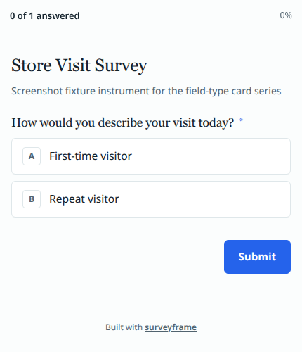
Real output of export_static_survey() for the visitor_type item: a progress indicator reading “0 of 1 answered”, the question marked required, two bordered option cards lettered A and B for “First-time visitor” and “Repeat visitor”, and a Submit button.

Write the analysis plan before you collect anything

Do this part deliberately. The plan below is declared now, attached to the instrument, before a single response exists. method = "frequency" with roles = list(variable = "visitor_type") tells surveyframe which table and chart to produce later. Why this order matters is its own post if you want the fuller argument.

instrument <- sf_instrument(
  title = "Store Visit Survey",
  version = "0.1.0",
  components = list(choices, item),
  analysis_plan = list(
    list(
      id = "RQ1",
      research_question = "What proportion of visitors today are repeat visitors?",
      family = "descriptive_categorical",
      method = "frequency",
      roles = list(variable = "visitor_type")
    )
  )
)

Run the plan against responses

In your own project this is read_responses() reading a CSV or Google Sheet. Here it is 140 rows of synthetic data standing in for real ones, generated once with a fixed seed so this page renders the same result every time. The exact file is downloadable as 09-single-choice-responses.csv, if you would rather point read_responses() at a real file than regenerate it.

set.seed(42)
n <- 140
responses <- data.frame(
  visitor_type = sample(c("first", "repeat"), n, replace = TRUE, prob = c(0.62, 0.38))
)

run_analysis_plan() reads the plan attached to instrument and executes exactly that plan. plots = TRUE turns on the optional ggplot2 layer new in 0.3.3.

results <- run_analysis_plan(responses, instrument, plots = TRUE)
rq1 <- results[[1]]

Table 3
Frequency Distribution of visitor_type

Value	Frequency	Percent
First-time visitor	78	55.7
Repeat visitor	62	44.3

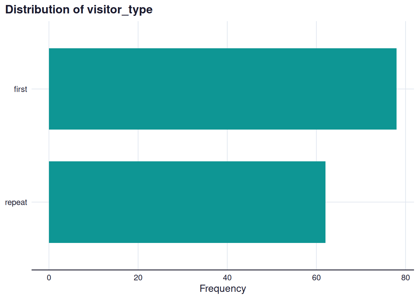
Frequency distribution for visitor_type (N = 140).

Every part of that table, chart and sentence was chosen before the numbers existed. method = "frequency" was decided in the plan section above, before responses existed.

Adapt this to your own survey

To reuse this for a different single_choice question, change three things and leave the rest:

1. The id and label in sf_item()
2. The values and labels in sf_choices()
3. The variable in the plan’s roles, to match your new id

Everything else, the codebook, the export, the plan structure and run_analysis_plan(), works the same way whatever the question asks.

Get surveyframe

install.packages("surveyframe")

• Documentation: mohammedalisharafuddin.github.io/surveyframe
• Source: github.com/MohammedAliSharafuddin/surveyframe
• Release notes: surveyframe 0.3.3 is on CRAN
• The reasoning behind the plan-first design: why the analysis plan comes first